Some neurological disorders, including stroke, spinal cord injury, and neuromuscular diseases, have been associated with disorders in human gait. Many researchers use physical therapy to help regain motor function in patients with such disorders. Gait training with body weight support systems have been used to improve ambulation in patients with spinal cord injury and paraplegic patients with little or no muscle activation [1,2]. Conventional gait training done manually by physical therapists is labor intensive, costly, and the number of sessions nowadays are increasingly limited by Medical Insurance Providers.

Although physical therapists try ato stay consistent in training, their efforts in trying to maintain the same pattern of gait motion training will differ from one therapy session to another. Measuring the treatment progress will be hard this way. Mechanical/robotic devices, such as Haptic Foot Device Trainers and Locomote systems, have been developed to provide consistent and efficient gait training [3-5]. Such systems cost a lot and not available in every rehabilitation center.

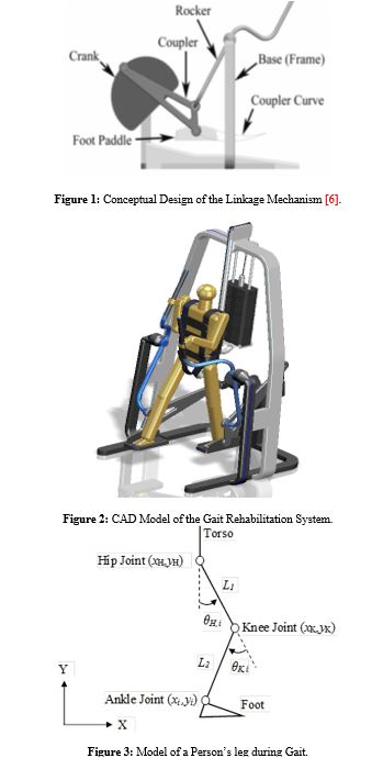
The research work in [6] describes the synthesis of a linkage mechanism system for Gait Pattern generation in a sagittal plane along with design of a motion control system. Features of this system includes consistent training, affordability, ability to measure patient’s performance, safer system, and easy of manufacturability. This paper introduced here first investigates the effect of using the gait rehabilitation system presented in [6,7] to train patients whose heights are different from the height that the system was designed for. A dimensional synthesis process of a linkage mechanism for gait pattern generation was introduced in [6,7]. This mechanism guides the user’s feet through a closed path formed with a coupler curve of the mechanism [8,9] to produce coordinated motion of the legs joints to follow normal physiological gait pattern [10], see (figure 1).

Other mechanisms have also been designed for gaiting training and some of them were discussed in [11]. Work presented in [11] has not discussed how a system that is dimensionally synthesized for one height affects the training if used for a person with different height, as well as how the person should be placed on the system to reduce any unfavorable effects. In order to understand the effect of mismatched height, the work presented in [6, 7] is first reviewed. Followed by an analysis of the effects, a methodology is then developed to determine the placement of patients for minimizing unfavorable effects caused by the mismatched height. The natural kinematics constraints of the mechanism produce trajectories that limit the knee and hip joints’ Range of Motion (ROM), thus improve the gait training safety [6]. Each patient’s height will have his/her own corresponding set of mechanism dimensions. The mechanism shown in figure 1 was synthesized using a person average height of 1.75 meter. If another patient with a different height is to be trained, the approach given in [6] allows the designer to find a new set of dimensions for this specific height and adjust the linkage accordingly. This approach can be applied for a system designed for any other nominal height as the closed path or coupler curve can be scaled. This does require the system to be designed to be dimensionally adjustable.

For a rehabilitation center that can only be equipped with systems at several nominal heights, it would be desirable to be able to train a range of patient heights with a system designed for a particular nominal height, even if the system is not adjustable. This way, a limited set of systems can be used to train a wide range of patients. The research work presented here is motivated by this desire. It starts with one set of link dimensions designed for a specific height and then analyze the effect on both the hip and knee joints profiles when a person with different height (either taller or shorter) is trained. The results of the analysis will be used to find a solution that optimize the placement of the patient to reduce the effect on both the hip and knee joints profiles. With the presented methodology, a range of heights can be determined for a given limit on the effect such that the patients within the range of heights can still be trained with a system designed for a particular nominal height.

            Investigating the effect of training people with heights different from an average value is considered first here. Using an average height of 1.75 m as an example to see the effect on both the hip and knee angle profiles. The effects are studied as two cases:

              (1) Heights higher than 1.75 m, and

              (2) Heights lower than 1.75 m.

                We will first consider the case with heights of the patients to be higher (Hg) than 1.75m (Havg).  The equations for obtaining the hip (θH) and knee (θK) angles are derived for establishing their angle profiles during a gait cycle.

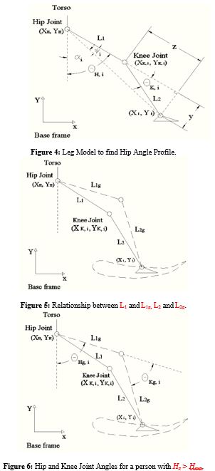
The position of the ankle joint relative to the coordinate frame shown in figure 3 is given from forward kinematics [7] by:

,  (i=1,⋯,51)                   (1)

Where xi and yi represent the coordinates of the ith point of the 51 ankle positions on the coupler curve. L1 is the length of thigh (from greater trochanter to knee) while L2 is the length of shank (from knee to ankle).   

                Re-writing the above equation, we get:                    

                ,  (i=1,⋯,51)                 (2)

                Squaring each line of equation (2) to get:

                ,  (i=1,⋯,51)   (3)

                Expanding each line, we get

                ,  (i=1,⋯,51) (4)

                Adding the two lines and collecting terms, we get:

                 (5)

               Using the trigonometric identities and , equation (5) becomes:

               (6)

or

                (7)

Expressing equation (7) in terms of , we get:

 (8)

which leads to:

(9)

and only the positive sign should be used since .

Now the hip angle can be calculated based on the geometric relation shown in the figure 4 using the following equations:

θH,i=(φi)+(αi) ,  (i=1,⋯,51)

θH,i=tan-1 [ yL1+z] +tan-1 [xi-xHyi-yH] ,  (i=1,⋯,51)

θH,i=tan-1 [L2×sin (θK, i) L1+L2×cos (θK, i) ] +tan-1 [xi-xHyi-yH]  ,  (i=1,⋯,51)                                                                                (10)

2. Training Patients Taller than the Average Height (1.75 m)

Let us consider the situation where a four-bar mechanism is dimensionally synthesized for gait training of people with heights at 1.75 meters. Their hip joints should be placed at certain coordinates (xH, yH) with respect to the global system or the base frame. The resulted coupler curve for guiding them foots is formed by points with coordinates (xi, yi) corresponding to the height of 1.75 meter. Considering placing a person of a height greater than 1.75 meter at the same hip location (xH, yH) and using the same four-bar mechanism and the same coupler curve, study of the effects on the hip and knee joints angle profiles is needed.

According to [12], the two leg lengths can have related to a Person’s total height as follows:

(11)

(12)

Since the total height will affect both L1 and L2, this difference in heights will change the values of angles calculated with equations (8), (9), and (10).

Consider a height greater (Hg) than 1.75 meter (Havg). Since Hg > Havg, we can write:

             (13)

Where will be greater than one since Hg > Havg. For example, if Hg =1.8 m, then =1.02857.

The lengths of leg segments correspond to height Hg are as follows:  

(14)

(15)

Substituting equation (13) in each of equations (14) and (15), we get:

(16)

(17)

Equations (16) and (17) can be re-written using equations (11) and (12) as follows:

(18)

(19)

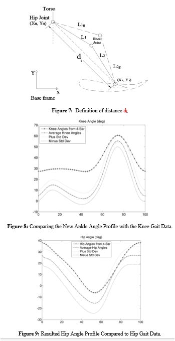
Since Hg > Havg, then is greater than one, and from equations (18) and (19), we can see that L1g is greater than L1 and L2g is greater than L2. The relationships between these lengths are shown in figure 5.

As mentioned earlier, we want to study the effects on the hip and knee joint angles if a patient having a height of Hg is placed at the same hip location (xH,yH) and using the same four-bar mechanism (same coupler curve (xi, yi)). The results of equation (8) can be used (since it’s have the same derivation) to study the effects of having larger leg length segments (L1g and L2g) and see what the new hip and knee joint profiles would be, namely, θHg and go, which are shown in figure 6.

Similarly, the relationship for the new knee angle, θKg can be derived as follows.

 ,  (i=1,⋯,51) (20)

The sum of the first two terms in the numerator expression represents the square of the distance between the hip location (xH, yH) and the current foot location (xi, yi). We will call this distance “di”, shown in figure 7.

Re-writing equation (20), we get:

,  (i=1,⋯,51) (21)

Note that for each foot (ankle) location (xi,yi), the distance “di” will differ, and thus cos (θKg, i) will also differ. Using equations (18) and (19), we can write equation (21) as:

,  (i=1,⋯,51) (22)

Dividing each of the numerator and the denominator by, we get:

,  (i=1,⋯,51) (23)

Comparing equation (23) with equation (8), we see that the net effect of training someone with a height of Hg using the same hip location and the same four bar mechanism results in dividing the first term in the numerator expression of equation (8) by. Since is greater than one, then the first term in the numerator expression of equation (23) will become smaller than the corresponding term in equation (8) and this will decrease the value of the cosine which will affect also the sine of the knee angle.

Similarly, equation 9 can rewritten as:

,  (i=1,⋯,51) (24)

According to equation (24), the decreased value of the cosine will increase the corresponding value of the sine, which means that the corresponding knee angle (θKg) will increase.  An increase in the knee angle will apply to all the foot locations. Thus, if we want to train a patient with a height greater than 1.75 meter using the same hip location and the same four bar mechanism, the net effect is that all the knee angles will be greater than those produced by the average height of 1.75 m.

Through an inverse kinematics analysis performed using a height of 1.8 meter as an example, the effect can be shown clearly in figure 8, as compared with the information on the hip and knee angles from the Clinical Gait Analysis Normative Gait Database [13]. Those values of the hip and knee angles are normalized during the gait cycle at 2% intervals. The average values were plot along with the standard deviated values. The curve that results from this inverse kinematics analysis is labeled as “Knee Angles from 4-Bar” in figure 8. The inverse kinematics results agree with the conclusion; that is the knee angles for 1.8 meter will be greater than those for 1.75 meter during the entire gait cycle.

The effect on the corresponding hip angles can be studied in a similar way. The new hip angle that corresponds to a height Hg can be obtained as follows:

θHg,i=(φg,i)+(αi)  ,  (i=1,⋯,51)

θHg,i=tan-1 [L2g×sin (θKg, i) L1g+L2g×cos (θKg, i) ] +tan-1 [xi-xHyi-yH]  ,  (i=1,⋯,51)                   (25)

Again, using equations (18) and (19) and substituting them in equation (25), we get:

,  (i=1,⋯,51) (26)

Cancelling out from the numerator and the denominator, we get:

,  (i=1,⋯,51) (27)

The second term in equation (27) is not affected by the lengths for the same hip and foot (ankle) locations. We know from equations (23) and (24) that height Hg would increase sin (θKg, i) and decrease cos (θKg, i) . These changes will increase the fraction in the first term of equation (27) which will increase θHg, i. The same inverse kinematics analysis used to find the knee angle values was used to find the corresponding hip angles and the results also show greater hip angles, as expected, see Figure 9.

The resulted conclusions make sense since training someone taller at the same hip location will cause the person to adjust by increasing both hip and knee angles to reach the same foot location that was used by a person whose height is 1.75 meter, as shown in figure 5.

To reduce these effects so that the hip and knee angles become closer to the average values from the Gait data, the hip location must be adjusted. Let us take a closer look at the previous equations.

In equation (21), we defined:

              (28)

A figure that shows how the square of the distance variable (di2) profile looks for one cycle for a height of 1.75 meter is shown in figure 10.

It was shown earlier in equation (23) that the net effect of using Hg would be to divide the first term in the numerator in the right-side expression of equation (23) (shown again below) by ∆h2.

If we have a height Havg (1.75 m), then ∆h2=1. But since we have Hg, then ∆h2>1 and the whole numerator expression will decrease. To make the value of the ratio of equation (23) be equal to that of equation (8) for the same ith location, we need to increase the value of di2 with a certain value. This increase can be done by referring to equation (28) where we can increase either the value of xH, YH, or both for the same ith location. In other words, to fix (by lowering) the hip and knee profiles, we need to find a new location for the hip joint in the base frame. We will define this new distance as di_n, defined by the below equation and also shown in the figure 11 along with a new hip location (xH_n, YH_n).

             (29)

At a new hip location,  cos (θKg, i)  can be expressed as:

              (30)

If we want equation (30) to be equal to equation (8) (i.e. we have the same cosine of the knee angle for the same ith location), then the ratio of (din2) to ∆h2 should be made equal to the original di2, see equation (31).

                                                                                                                          (31)

Substituting equation (29) in equation (31) and re-arranging terms, we get                  

                                                                       (32)

This represents 51 equations with two variables: xH_n and YH_n. We can assign one value for one variable (YH_n for example) and solve for the other variable; XH_n. It can be seen that we have infinite number of choices for the value of the YH_n variable. The resulting equation will be quadratic in XH_n and so, we will have two solutions for XH_n for each YH_n. The suitable solution will be chosen.

Expanding equation (32) to get:

(33)

Note that this over all process of solving for the new hip location depends on our choice of selecting a value for di from figure 8, i.e., the hip location is solved based on one certain ith location. Since we have 50 unique locations in total, there are 50 choices for di to choose from. However, only one location is needed to be chosen since we seek only one new location for the hip joint. While this choice, as will be shown, will be suitable for that ith location, it will not be suitable for all values, i.e., the hip and knee angles at other locations will not be controlled, as will be shown later.

If we choose the first value of di from figure 10 and we choose (assign) a value for YH_n, where we will shift it up by 0.02 meters, then, solving equation (33) for XH_n would result in a shifted value of the hip by 0.0156 meters to the left. Originally, the hip location in the base frame had the coordinates of (0.8426, 0.4520) meters, and the new required location of the hip would be (0.82703, 0.4720) meters. However, it should have mentioned that there is a limit to how far the hip can be shifted in the vertical direction as the solution for inverse kinematics of the hip and knee angles puts a constraint on this. In other words, the foot needs to be close to the coupler curve and not be shifted up too much. Figure 12 shows the square of the new distance (di_n) using the above new hip location.

The values in this figure must be divided by ∆h2 (see equation (31)) and the new vector is called dig2. This vector is compared with the original di2 (from figure 10) in figure 13. The resulted hip and knee profiles are also shown in the figure.

The goal here, as can be seen from equation 31, is to make the ratio on the left side equal to that of the right side for a given ith location. Since the first location was chosen as an example, we can see that the two curves di2and dig2 in figure 13 are exactly equal at the first location (index one) as they were forced to be equal. However, we do not have a control over the other values. A closer look at the same figure shows that around 20% of the gait cycle, the dig2 curve starts to deviate from the di2 curve and this continues till they meet again around 90%. This is reflected on the hip and the knee profiles as can be shown in figure 13. The joints profiles using the new location will also start to deviate (around 20%) and meet again (around 90%).

Examining the two curves di2and dig2 in figure 13, we can see that the values for dig2 actually decrease starting around 20%. This decrease will cause the expression in equation (30) to be less than what it should be and this will make the knee angle increase, as can be seen in the knee profile in figure 13.

The same argument applies to the hip profile as an increase is noticed in the values between around 20% till 90% of the gait cycle. Thus, if we are able to make the dig2 curve closer to the di2 curve, the resulted hip and knee profiles will get closer to the desired values. Choosing a different vertical offset distance for the hip like +0.01 meters (shift hip upward) would result in the need to shift the hip in the horizontal direction by -0.03662 meters (shift hip to the left). Figure 14 below shows the resulted dig2 curve compared to the di2 curve, and the resulted hip and knee profiles.

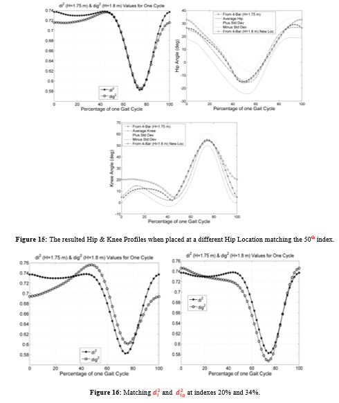
It can be seen that because of the larger deviation of dig2 curve compared to the deviation in figure 13, the resulted hip and knee profiles have more deviations than those in figure 13. Note that this analysis is done so di2 and dig2 curves still intersect at the first location in the gait cycle (i.e.: first index). Another location can be chosen in the gait cycle to make di2 and dig2 curves intersect, for example, at 50 % of the gait cycle. A choice of a vertical offset of 0.02 meters is made, and the resulted horizontal shift is found to be 0.01745 meters. The resulted hip and knee angle profiles are shown below.

The di2 and dig2 curves intersect at 50% of the gait cycle (as expected) and they deviate in the regions between 0% and 40% and also at the end of the gait cycle and this is reflected on both the joints profiles. It is worth to mention that deviations in the knee joint profile will be more visible and noticeable than in the hip and joint profiles as equations (30) and (31) are related to the cosine of the knee joint profile. The better that matching of di2 and dig2 curves is, the better the knee joint profile is, and vice versa. This can be seen in all cases.

Another location is chosen to where di2 and dig2 curves intersect, 34% of the gait cycle. The result is shown in the left of figure 16. For this case however, the values of  dig2 curve start to increase in the interval between 34% and till around 48% of the gait cycle. These large values cause the cosine in equation (30) to be larger than one for any point in this interval. The inverse kinematics analysis will not be able to solve the corresponding hip and knee angles; as the cosine of any angle should be only between -1 and 1. By going back to figure 11, this means we have large distance requirements for this interval and the ankle joint (foot) will not be able to reach the coupler curve. Several values for the vertical shift were tested and all gave same result as above. As another example, the two curves are made to intersect at 20% and the result is shown on the right of figure 16. Also, here, there were values where the inverse kinematics analysis was not able to solve the corresponding hip and knee angles. This means that we cannot have a solution at any index.

It is noted that whenever at least one value of dig2 vector is larger than the maximum value of di2 curve, an inverse kinematics solution cannot be solved. By referring to equation (30), this means that the value of the cosine of the knee angle is greater than one and thus the inverse kinematics cannot be solved.

Instead of choosing both an arbitrary value for YH_n and an index in the gait cycle (to make di2 and dig2 curves intersect) and then solve for XH_n, an optimization process can be performed to choose an optimal hip location (for each) such that this location will minimize the distance between the two curves. The optimization process can be done using the least square method [14], [15], and [16] which will minimize the square of the distance between the two curves for a given.

First an objective function is needed. By referring back to equations (31) and (32), the objective function is defined below:

                                                                (34)

This nonlinear objecting function is to be minimized. Note that each of xi, yi and di, is a vector of size 51 elements. Note also that the optimal hip location (XH_n, YH_n) will correspond to a certain. If we have a different (a patient with a different height), then we need to perform the optimization process again to find the optimal hip location that corresponds to this.

The nonlinear optimization process can be implemented in MATLAB using the function LSQNONLIN which solves nonlinear optimization problems. An initial guess is needed as an input for this function. A code in MATLAB is written and the needed vectors: xi, yi and di are passed to the function LSQNONLIN. The current along with an initial guess need to be passed also to the function LSQNONLIN. As a check, if is set to one (we have a height of 1.75 meters), then the code should return the original location (0.8426 m, 0.4520 m), which it does.

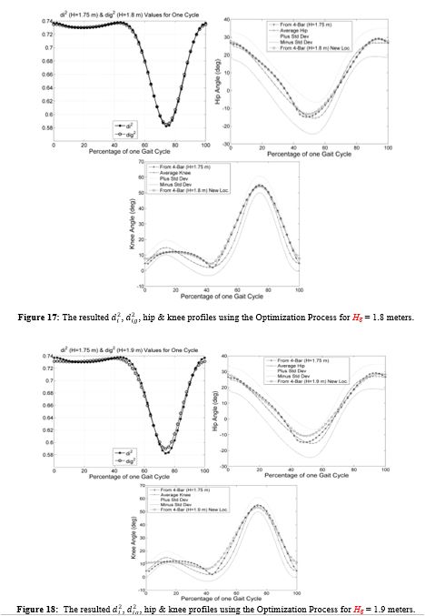
In the next figures, the results of the optimization process for different heights (or different) are shown. For example, for Hg = 1.8 meters, the optimal hip location is: (0.8415 m, 0.4770 m). Note that there is a vertical shift to compensate for the increase in the height. A comparison of two curves di2 and dig2 along with the resulted hip and knee profiles are shown in figure 17.

It is noted that dig2 curve is following di2 curve much better than all the previous cases shown in figures 12 through 16, which is also reflected well on the resulted hip and knee joints profiles.  For Hg = 1.9 meters, the optimal hip location is: (0.8391 m, 0.5267 m). A comparison of the di2 and dig2 curves along with the resulted hip and knee profiles are shown in figure 18.

For Hg = 2 meters, the optimal hip location is: (0.8363 m, 0.5762 m), and the corresponding figures are shown in figure 19.

The effect of the deviation of the dig2 curve from the di2 curve at the start and end of the gait cycle and around 45 % of the gait cycle is reflected in the knee joints profile. The hip joint profile is less sensitive than the knee joint profile for such deviations; a fact that can be checked in all previous figures.  For Hg = 2.2 meters, the optimal hip location is: (0.8298 m, 0.6746 m). A comparison of the dig2  and di2 curves along with the resulted hip and knee profiles is shown in figure 20.

All of the previous cases were derived for a height of a person that is greater than the average height (1.75 m). The optimization process should now be applied for heights less than 1.75 meters to find an optimal hip location. These heights will be represented by Hs.

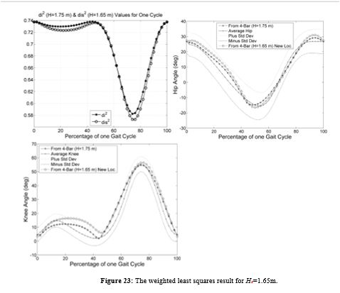
For Hs = 1.65 meters, the optimal hip location can be found with the same optimization procedure as (0.8445 m, 0.4020 m). The resulted squared distance between hip joint and ankle joint is referred to as dis2. A comparison of the di2 and dis2 curves is shown in the left plot in figure 21. It can be seen from the figure that there are certain points where values of the dis2 are greater than the maximum of the di2 curve, specifically around 1% and 50% of the gait cycle. Since these points are near the inverse kinematics singularity, inverse kinematics cannot be performed at some of these points if the hip is placed at the calculated optimal hip location. The same problem can also be seen in the case of Hs =1.55 meters, as shown in the right plot in figure 21. Since this produces unreachable coupler points, the optimization procedure must be revised to find alternative objective function.

Since the objective function is nonlinear in terms of the hip locations coordinates: XH_n  and YH_n, the weighted least squares principle [17] for nonlinear systems is proposed where weights are applied around critical locations to make the error smaller compared to the unweighted locations. In the case of figure 21, weights can be applied around 1% and 50% of the gait cycle to try to make the dis2 curve closer to the di2 curve.

Since the equations are nonlinear, the procedure requires an initial guess for the hip location. Adjustments [17] to the initial guess will be calculated using:

                     (35)     

And then these adjustments are added to the initial guess hip location and iteration is repeated till the adjustments converge to some chosen value. A value of 10-15 is chosen. The matrices in equation (35) are defined in [17] as follows:

∆X is a vector that has adjustments (dXH_n  and dYH_n) to the unknowns XH_n  and YH_n.

J is the Jacobian Matrix which contains the coefficients of the linearized observation equations [17].

JT is the transpose of the Jacobian matrix.

K is a vector that has the residuals.

The matrices are defined below.

Note “m” is 51 and the objective function Fi is evaluated from equation (34) at each xi and yi, for i = 1 to 51. The Jacobian matrix contains the partial derivatives of the objective function Fi with respect to the variables XH_n  and YH_n. Specifically, the Jacobian matrix is written as follows:

        (36)   

And the residual matrix is written as follows:

       (37)

In figure 21, locations around 1% and 50% had values that caused the singularity in inverse kinematics therefore insolvable. After applying weights at these locations, the dis 2values at these locations become lower as seen in figure 22 for Hs=1.55m. Optimal hip location using the appropriate weights is found to be (0.8480 m, 0.346 m). Figure 22 also shows the resulted hip and knee joints profiles.

It is noted that as the height gets closer to 1.75 meters, the solution of the curve will produce better hip and knee joints profiles. For example, the joints profiles in figure 23 for Hs = 1.65 m are much better than the joints profiles in figure 22 for Hs = 1.55 m.

           The research work presented here allows adjustments by finding an optimal hip location for a person whose height is different from what a gait generation mechanism was originally designed for. This will allow rehabilitation centers to have few number of mechanisms but still be able to train persons in a wide range of heights. The ranges shown here were just examples to show that the methodology works. The methodology is developed through an exemplary mechanism designed for training a person whose height is 1.75 meters. With the presented optimization procedure, it was shown how the optimal hip locations can be obtained for heights from 1.55 meters to 1.95 meters (as examples), but more research work will be needed to choose the range of heights that can be trained with a height like 1.75 meters, for example. If another mechanism is designed for a height of, let us say 1.35 meters, then it could be used to cover certain range of heights as 1.15 m to 1.55 meters and so on. Future research of this work would also involve designing physically the way by which the patient’s hip can be positioned and moved to the optimal hip location calculated by the methodology shown here.

1. Hesse S, Bertelt C, Jahnke MT, Schaffrin A, Malezic M, et al. (1995) Treadmill Training with Partial Body Weight Support Compared with Physiotherapy in Non-ambulatory Hemiparetic Patients. Stroke 26: 976-981.
2. Visintin, M, Barbeau H, Korner-Bitensky N, Mayo NE (1998) A New Approach to Retrain Gait in Stroke     Patients Through Body Weight Support and Treadmill Stimulation. Stroke 29: 1122-1128.
3. Jezernik S, Colombo G, Keller T, Frueh H, Morari M (2003) Robotic Orthosis Lokomat: A Rehabilitation and Research Tool. Neuromodulation 6: 108-115.
4. Schmidt H, Hesse S, Bernhardt R, Krüger J (2005) HapticWalker: A Novel Haptic Foot Device. ACM  Transactions on Applied Perception 2: 166-180.
5. Westlake KP, Patten C (2009) Pilot Study of Lokomat versus Manual-Assisted Treadmill Training for Locomotor Recovery Post-Stroke. Journal of Neuroengineering and Rehabilitation 6: 18.
   
6. Zhiming Ji, Yazan Manna (2008) "Synthesis of a Pattern Generation Mechanism for Gait Rehabilitation". Journal of Medical Devices 2 (3).
7. Yazan A. Manna, Fen Du, Zhiming Ji (2012) "Motion Control and Coordination in the Development of a Gait Rehabilitation System", Journal of Mechanical Engineering Science. Proceedings of the Institution of Mechanical Engineers. 226: 1885-1895.
8. Waldron KJ and Kinzel GL (1999) Kinematics, Dynamics, and Design of Machinery. New York: John Wiley & Sons (1999).
9. Mallik AK, Ghosh A and Dittrich G (1994) Kinematic Analysis and Synthesis of Mechanisms. Ch. 9, Boca Raton: CRC Press, 1994.
10. Whittle, MW. Normal Gait. In: Gait Analysis - An introduction 4th ed. Butterworth-Heinemann, 2007.
11. Zhongxia Xiang, Yixin Shao, Haitao Liu, Lili Li (2016) “Conceptual Design and Dimensional Synthesis of Cam-Linkage Mechanisms for Gait Rehabilitation”. Mechanism and Machine Theory 104: 31- 42.
12.  Winter DA (1979) Biomechanics of Human Movement, New York: Wiley, 1979, p.48.
13. Clinical Gait Analysis Normative Gait Database. Retrieved April 23, 20185 from the World Wide Web: http://www.clinicalgaitanalysis.com/data/
14. Chapra SC and Canale RP (2002) Numerical Methods for Engineers with Software and Programming Applications. 4^th edition. McGraw-Hill Higher Education, 2002.
15. Ramsay JO and Silverman BW (2005) Functional Data Analysis, 2^nd edition. New York: Springer
16. Robinson, Enders A (1981) Least Squares Regression Analysis in Terms of Linear Algebra.
17. Charles D. Ghilani (2010) Adjustment Computations: Spatial Data Analysis, Fifth Edition. John Wiley & Sons, Inc. 2010. Ch. 11, pages 178-204.