 research article
 Using Gray Relational and Artificial Neural Network in Insole Design and Development for Diabetes
Ching-Hu
Yang*, Chung-Shing Wang
Department
of Industrial Design, Tung-Hai University, Taichung, Taiwan
*Corresponding
author: Ching-Hu
Yang, Department
of Industrial Design, Tung-Hai
University, Taichung, Taiwan. Tel: +886932967688;
Email: gemlake@ms31.hinet.net
Received
Date: 24
September, 2018; Accepted Date: 6 October,
2018; Published Date: 16 October
2018
Citation: Yang CH, Wang CS (2018) Using Gray Relational and Artificial Neural Network in Insole Design and Development for Diabetes. Adv Res Foot Ankle: ARFA-107. DOI: 10.29011/ ARFA-107.100007.
1. Abstract
The purpose of this research is to design Insole for the diabetic patients. Using the multiplex system analysis, it compares the foot pressure data of 20 testers (Including a Diabetic Patient) plus insole measurement with six different materials and shapes to obtain the best diabetic shoes. In addition to the detailed discussion of the application of various methods in this unit, the questionnaire is also used. Based on these, the biomechanical experiments are used between patients and healthy people to prove the theory of this method’s feasibility.
Taking The “Comfort Rating” of diabetics is the research direction. General products of clinically-used foot treatment insoles are used to design a “Grey Relational” assessment model which is based on foot pressure measurement as the precondition. The model used is to find the most relevant insoles and foot shapes as practicing samples for “Artificial Neural Network (ANN)”. Through multiple iteration calculations and automatic grouping of the data input the most suitable patient insole pattern will be found from the samples. Then, the selected pathological insole as well as its design features are to be analyzed and discussed in detail for subsequent research, development and design.
2. Keywords: Diabetic Insole; Design Feature Foot Pressure Measurement; Grey Relational; Neural Networks
3.
Introduction
3.1. Motivation and Purpose
According
to the report issued by the World Health Organization (WHO) in 2016, the number
of patients has tripled from 1980 to 2014, up to 4.22 billion people. In
addition, according to the International Diabetes Federation (IDF), the global
medical cost of diabetes 2017 was about 0,7 trillion dollars, accounting for
12% of global medical expenditure. It is estimated that it will reach 0,9
trillion dollars in 2040. Boulton [1] believes that diabetic patients account for
approximately 50% of all non-traumatic lower extremity amputations, Gordois [2] study shows that diabetic foot ulcers are caused by
neuropathy or vascular ischemia. Among them, about 65% of foot ulcers are
caused by neuropathy. From these literatures, we know that foot ulcers not only
affect the quality of life of patients, but their pathogenesis often leads to a
regrettable outcome. The prevention of foot ulcers has become a vital issue
today [3].
About
10% of people with diabetes who suffer ulcers during illness are caused by
increased pressure in the shoes. Armstrong, [4], in its study
indicates that wearing a specific design of the footwear, the patient’s
worsened condition can be reduced during the follow-up care. Maciejewski, et al, [5], from the
pathological literature, it stresses the importance of wearing a therapeutic shoe
to prevent ulcers. Knowing that footwear is the main prevention; the content
specifically mentions that the design of the relevant medical footwear is one
of important Influencing factors.
All
studies indicate that wearing a pair of comfortable insoles is important to
prevent diabetic patients from getting worse. The special diabetes insole can
reduce the foot pressure to a certain extent and prevent the wear of foot skin.
It is also designed to provide good foot support and improve the patient’s balancing
capability while walking.
To
design shoes for diabetic patients, the first thing is to avoid the risk of
getting foot ulcers. The rising foot pressure may be caused by improper design
of the inner space of the shoe and improper selection of materials. The
increase in temperature and humidity may easily lead to ulcer. Therefore, the
main goal of designing shoes for diabetic patients are to reduce the pressure
on the sole and create a comfortable interior space [6].
Although
the CAD system for manufacturing models of shoes has been developed, two major
shortcomings remain which limit the applicability and production of footwear.
First, they do not have any follow-up system to organize and support the data
of diabetic patients. In other words, there is no database for patients.
Secondly, there is no standard measurement system to follow so the risk of
ulceration can be reduced. Considering the factors of normal foot care, medical
expenses and wearing comfort, this study is proposing an intelligent analysis
system to find insole design features for diabetic patients. Based on patient
foot pressure data and shoe samples, specific comfort fits are calculated and
analyzed so a patient can find a suitable insole and reduce the risk of ulcers.
3.2. Research Limit
Based
on the study of Chapman [7], it is recommended that the feet of
patients with neuropathy need to travel slowly and exercise regularly. It has
been known that patients with diabetes can’t walk fast, so the angle of heel
movement and toe elasticity measurement
is not to
be discussed in
this study. Since, he
foot pressure measurement experiment is also based on the fixed-point
standing measurement, therefore, the walking test is not to be conducted. In
addition to Dynamic pressure measurement, because the sensitivity of the
machine measurement gasket has its limitations, the length of the data
transmission line has its limitations, and the lengthy experiment time may affect
patients’ psychological reaction, and the gait measurement and analysis are not
available, the correct gait measurement and analysis cannot be acquired, so it
is not being used [8].
The
diabetic patients whose lesions are not developed are selected in this study.
Based on the Wagner classification, one patient with minor symptoms can be
defined as grade 0 and is the best candidate to be tested. Those people with
grade above 0 may not be tested because they may already have ulcers. The
adoption of this method has the following reasons: the needs of patient’s care;
the cost of pathological footwear; and most importantly, the concept of
“prevention is better than cure” [9].
Diabetic
patients often use their own subjective feeling to decide if the insoles are
comfortable. From the concept of” Human Factors
Engineering “it may be adequate. But from scientific viewpoints this kind of medical
treatment is not enough for patients. The poor blood circulation of limbs
caused by diabetes which affects the sensitivities of skin cannot be used to
judge the fitness although the shoes may be felt comfortable by patients.
Therefore, a comfortable and correct insole requires an objective and
scientific way to correct all problems. This is another reason why
questionnaire about comfort answered by patients should be avoided. Measurement
seems to be the solution.
4.
Methods
In
this study, the Grey Relational evaluation model was designed based on the “Comfort
of Diabetic Patients” to find out the most relevant insole style in the foot
and insole samples. As the most suitable insole option, this result will be
used as a follow-up. The training of the Artificial Neural Network (ANN) is
evidenced. The research process is described as (Figure
1).
4.1. Experimental Design: Neural Network Learning Parameter Design
In
order to verify the learning of “Back-Propagation Neural Network”, the Matlab
program simulation is performed for the recognition and grouping problem of 2D
graphics according to the inverse transfer learning algorithm of “the Gradient
Steepest Descent Method”. First prepared a set of five different original
patterns (Figure 2), converted to grayscale
patterns (Cat, Squirrel, Rabbit, Chicken, Bird) through Mat lab calculations,
and used these samples as a network reference. For the sample, each pattern is
defined by the grayscale value of the 12×12 matrix, and the original grayscal e
pattern is shown in (Figure 3) The grayscale
value is a real value between 0 and 1, when the grayscale value is 0, it is
defined as white; the grayscale value is 1, it is defined as black. In order to
facilitate the calculation of network learning, we also adjust each pattern to
a 144 × 1-line vector pattern.

 is the number of neurons in the
output layer.
is the number of neurons in the
output layer.
3.
Introduction
3.1. Motivation and Purpose
According
to the report issued by the World Health Organization (WHO) in 2016, the number
of patients has tripled from 1980 to 2014, up to 4.22 billion people. In
addition, according to the International Diabetes Federation (IDF), the global
medical cost of diabetes 2017 was about 0,7 trillion dollars, accounting for
12% of global medical expenditure. It is estimated that it will reach 0,9
trillion dollars in 2040. Boulton [1] believes that diabetic patients account for
approximately 50% of all non-traumatic lower extremity amputations, Gordois [2] study shows that diabetic foot ulcers are caused by
neuropathy or vascular ischemia. Among them, about 65% of foot ulcers are
caused by neuropathy. From these literatures, we know that foot ulcers not only
affect the quality of life of patients, but their pathogenesis often leads to a
regrettable outcome. The prevention of foot ulcers has become a vital issue
today [3].
About
10% of people with diabetes who suffer ulcers during illness are caused by
increased pressure in the shoes. Armstrong, [4], in its study
indicates that wearing a specific design of the footwear, the patient’s
worsened condition can be reduced during the follow-up care. Maciejewski, et al, [5], from the
pathological literature, it stresses the importance of wearing a therapeutic shoe
to prevent ulcers. Knowing that footwear is the main prevention; the content
specifically mentions that the design of the relevant medical footwear is one
of important Influencing factors.
All
studies indicate that wearing a pair of comfortable insoles is important to
prevent diabetic patients from getting worse. The special diabetes insole can
reduce the foot pressure to a certain extent and prevent the wear of foot skin.
It is also designed to provide good foot support and improve the patient’s balancing
capability while walking.
To
design shoes for diabetic patients, the first thing is to avoid the risk of
getting foot ulcers. The rising foot pressure may be caused by improper design
of the inner space of the shoe and improper selection of materials. The
increase in temperature and humidity may easily lead to ulcer. Therefore, the
main goal of designing shoes for diabetic patients are to reduce the pressure
on the sole and create a comfortable interior space [6].
Although
the CAD system for manufacturing models of shoes has been developed, two major
shortcomings remain which limit the applicability and production of footwear.
First, they do not have any follow-up system to organize and support the data
of diabetic patients. In other words, there is no database for patients.
Secondly, there is no standard measurement system to follow so the risk of
ulceration can be reduced. Considering the factors of normal foot care, medical
expenses and wearing comfort, this study is proposing an intelligent analysis
system to find insole design features for diabetic patients. Based on patient
foot pressure data and shoe samples, specific comfort fits are calculated and
analyzed so a patient can find a suitable insole and reduce the risk of ulcers.
3.2. Research Limit
Based
on the study of Chapman [7], it is recommended that the feet of
patients with neuropathy need to travel slowly and exercise regularly. It has
been known that patients with diabetes can’t walk fast, so the angle of heel
movement and toe elasticity measurement
is not to
be discussed in
this study. Since, he
foot pressure measurement experiment is also based on the fixed-point
standing measurement, therefore, the walking test is not to be conducted. In
addition to Dynamic pressure measurement, because the sensitivity of the
machine measurement gasket has its limitations, the length of the data
transmission line has its limitations, and the lengthy experiment time may affect
patients’ psychological reaction, and the gait measurement and analysis are not
available, the correct gait measurement and analysis cannot be acquired, so it
is not being used [8].
The
diabetic patients whose lesions are not developed are selected in this study.
Based on the Wagner classification, one patient with minor symptoms can be
defined as grade 0 and is the best candidate to be tested. Those people with
grade above 0 may not be tested because they may already have ulcers. The
adoption of this method has the following reasons: the needs of patient’s care;
the cost of pathological footwear; and most importantly, the concept of
“prevention is better than cure” [9].
Diabetic
patients often use their own subjective feeling to decide if the insoles are
comfortable. From the concept of” Human Factors
Engineering “it may be adequate. But from scientific viewpoints this kind of medical
treatment is not enough for patients. The poor blood circulation of limbs
caused by diabetes which affects the sensitivities of skin cannot be used to
judge the fitness although the shoes may be felt comfortable by patients.
Therefore, a comfortable and correct insole requires an objective and
scientific way to correct all problems. This is another reason why
questionnaire about comfort answered by patients should be avoided. Measurement
seems to be the solution.
4.
Methods
In
this study, the Grey Relational evaluation model was designed based on the “Comfort
of Diabetic Patients” to find out the most relevant insole style in the foot
and insole samples. As the most suitable insole option, this result will be
used as a follow-up. The training of the Artificial Neural Network (ANN) is
evidenced. The research process is described as (Figure
1).
4.1. Experimental Design: Neural Network Learning Parameter Design
In
order to verify the learning of “Back-Propagation Neural Network”, the Matlab
program simulation is performed for the recognition and grouping problem of 2D
graphics according to the inverse transfer learning algorithm of “the Gradient
Steepest Descent Method”. First prepared a set of five different original
patterns (Figure 2), converted to grayscale
patterns (Cat, Squirrel, Rabbit, Chicken, Bird) through Mat lab calculations,
and used these samples as a network reference. For the sample, each pattern is
defined by the grayscale value of the 12×12 matrix, and the original grayscal e
pattern is shown in (Figure 3) The grayscale
value is a real value between 0 and 1, when the grayscale value is 0, it is
defined as white; the grayscale value is 1, it is defined as black. In order to
facilitate the calculation of network learning, we also adjust each pattern to
a 144 × 1-line vector pattern.
is the number of neurons in the
output layer.
4.2
Design Element:
Pathological
insole comfort design insole design, most of them use image capturing equipment
to obtain the three-dimensional contour data of the foot, and then make partial
modifications according to the individual's physiological condition by
professional technicians or doctors. According to the modern point of view, the
above design pattern is more subjective and subjective, that is, experience. As
a benchmark for the evaluation of design decisions, the law is biased. A pair
of comfortable diabetes insoles need to have the following features and needs:
(1).
wearing fit and even distribution pressure. (2). Decompression and soothing for
local pain (3). adjust the stability of the body to static posture and
movement. (4). The pressure can be balanced (5) insole material and angle
adjustment to achieve the shock absorption effect. (6). The medical expenses
required are lower and safer than other treatments. (7). Can alleviate sore
problems.
4.3. Research Method Execution
In
view of the above-mentioned medical insole design requirements, the
physiological foot pressure is used as the basis for measurement, and an
objective comfort evaluation model is established to replace the traditional
expert rule to calculate the insole comfort. To explore the comfort correlation
between the patient's foot and the "insole"
This
study addresses the needs of the research topic and divides method execution
into the following three steps.
4.3.1.
Biomechanical
Experiment Planning
The
biomechanical experiment aims to explore the type of insole used by the
tester's foot, which can achieve the pressure of a certain dispersion and
reduction in a certain block, and use it as a case for the subsequent
evaluation of the comfort of gray theory.
4.3.1.1.
Physiological
Experiment Variables and Design Planning
This
experiment mainly analyses the comfort evaluation of the tester's foot
pressure, in order to find the insole form suitable for the tester. The total
number of experimental samples is 20, including one primary diabetic patient,
the experimental object is male over 20 years old, and the weight is not
limited. The sample number is from A-U (including R patients with diabetes). The
experimental materials are commercially available male full-pad insoles, totalling
6 models, with the main function of reducing the foot pressure, which can be
tailored according to the foot type of self-cutting, increase the wearing
comfort, and avoid the pain position to be hurt again, it is classified as
thick, thin, soft, hard, and supported by the upper and lower arches. In order
to assort the limitations and accuracy of the foot pressure test pad, the size
is the suitable for those who wear the (American) specifications 7 to 11, The
sample characteristics are as follows (Table 2) (Table 3).
The
experimental site is located in Taiwan Taichung Shoes and Sports Leisure
Technology R&D Center (Shoe Technology Centre). The foot mechanics
experimental equipment of this study is Tek-Scan contact pressure measurement
pad. The hardness measurement data is measured by the Shore C Hardness of six
times. Using the German GEMMETER measurement.
4.3.1.2.
Experimental
assumptions
According
to the literature, when the plantar contact area changes, the foot pressure
will reflect different data, so this experiment assumes that different styles
of insole style will affect the distribution of interface pressure, and the
insole style is closer to the foot Type, the total pressure and peak value will
also decrease, and the contact area will increase. Praet [10] believes that the height of the arch is linear
with the pressure of the foot, while the thickness of the insole increases and
the peak pressure of the heel also decreases. According to the theory, the
thickness of the insole No. 2 selected in this experiment is increased, the No.
3 insole has a thickened arch function, and the No. 5 insole particularly
strengthens the insole arch and heel thickness and hardness.
Most
scholars have proposed The influence of the foot pressure parameters also
includes the area of contact. When the plantar contact area changes, the foot
pressure will reflect different data. All experiments are carried out using a
full-touch insole. It has a considerable effect on reducing foot pressure. Therefore,
this experiment uses the full-foot touch insole, and the half-type insole is
not used. The literature also proposed that the peak pressure of the general
foot Should fall in the palm area and near the heel. The diabetic patients are
more obvious. This experiment also sets the same research hypothesis, so that
the follow-up results can be used as a verification and discussion [11].
4.3.1.3.
Experimental
Limitations
The
number of full-pressure test is more than 4 times, but in the end, only the complete
4 of the image files are adopted, and the average value is calculated (the shoe
technique expert has precluded the foot pressure type with large defect). The measurement of the experiment only uses
the right foot. Due to research constraints, and most of the customary are
right feet, that is the subject of discussion. Although this effect has lost
effectiveness, the strict requirements and consistency of the measurement
posture can make up for its lack.
4.3.1.4.
Experimental
Procedure
The
experiment consists in measuring the pressure distribution of the tester's
static stepping on different styles of insoles, obtain five pressure parameter
data: Pressure Peak (PP), Pressure-Time Integral Value (PTI), contact area, Power
Peak (PF), Power-Time Integral Value Data (FTI), total Measured more than 4
times. The measurement method adopts a one-way static measurement, and the
insole is fixedly placed in a pre-planned position for the tester to measure in
the bare foot state, in order to express in a clear and simple manner, the
experiment is performed by computer image type. (Figure
5a,b).
˙The
various foot pressure measurements and min and max data are in the (right
window) and the graph is in the (middle window) foot pressure map (left window)
as follows. The pressure type of each foot type and the insole, through the
expert experience, the pressure pattern of 4 times or more is selected, the
bare-foot measurement of the S-tester is taken as an example to deduct the bad
pressure pattern. After only four of the pressure samples (Figure 6) were adopted as the follow-up data. Finally,
through the internal automatic calculation function and Foots can software to
obtain the pressure parameters are used for subsequent comfort evaluation
calculations, the optimal insole selected for comfort evaluation can be
converted into matrix form for the “optimal insole grouping” of this study.
4.4. Comfort Evaluation:Application of Grey Relation Theory
Using
human foot pressure data to explore unclear comfort information, this method is
in keeping with the concept of Grey theory, "external information is clear,
but internal information is not clear" and "for uncertainty, multivariate
input, scatter data Do effective processing”. This means that in the absence of
information, this study will use gray correlation to derive the essence of the
system and get the best answer [12].
4.4.1.
Comfort
Evaluation Mode Establishment
In
order to achieve the goal, this study uses the Matlab program to perform the
comfort evaluation calculation. The method is to analyse the pressure parameter
data of the mechanical experiment by statistical average method, the pressure
parameters are presented in a matrix, and Normalize the processing, select the
large value and the small value of each pressure parameter to define a new
reference sequence. After completing the above steps, calculate the distance of
the original sequence. And new reference sequence and set the recognition
coefficient ζ0.5. Further, the Gray relation coefficient
is calculated, and the relation degree is determined. The calculation process
is as follows (Figure 7).
4.4.2.
Comfort
Evaluation Calculation
By
the association of variables and parameters as the basis for calculating the
degree of Grey relation, the steps are divided into six major items, including
a. defining the pressure parameter sequence, b. normalizing the pressure
parameters, c. defining a new reference sequence, d. calculating the gray
relation distance, e. Calculate gray relation coefficient, f. Calculate gray
relation degree and sequence.
4.4.3.
Comfort
Evaluation Test Certificate
From
the table (Table 4,5), the Gray relation
calculated according to the six insoles and the optimal insole sorting the No.
2 insoles that are best for the feet of
most experimenters., because the initial screening of the sample insole is
Experts recommend classification according to the difference between thick,
thin, soft, hard and support positions. Mainly to verify the different
functions of each sample insole, did not expect this experimental result, in
order to more accurately find a suitable insole difference for each tester,
this study will move the No. 2 insole, remaining five The insole is again
subjected to gray relation analysis and calculation, obtain the optimal insole
sorting of the tester's second experiment, and also to find the insole suitable
for diabetic patients, and to analyse the final result (Table
6,7).
The underline of the data is
Gray-relation data. Among the six insoles the data in red are the most suitable
ones for diabetics. The data in blue the second best.
In order to get more detailed sorting,
the No. 2 insole for all testers is removed in this Table. ̇The underline
numbers are gray-relation data. The red data is the most suitable for diabetics.
4.4.4.
Analysis
of Grey Relation Results in Comfort Evaluation
From
(Table 5), the optimal insole sorting of the six
insole Gray relation is ranked. The No. 2 insole is most suitable for the feet
of most experimenters. The No. 2 insole is the thickest and Medium hardness in
all insoles. In order to contact the plantar area, it has a flat shape, so it can
be moulded according to the shape of the individual's foot. It is a modern
latex material, also called a memory material. Through experiments, this type
of insole can best reduce the impact of foot pressure. From this point, it can
also be proved that the increase in the thickness of the insole mentioned by Livery [6] will
directly affect the pressure of the sole and achieve the
Verification
(Table 6,7) are the best insole rankings. we can
find that the ranking of the insole No 2 is discarded. It does not mean that
its position will be replaced by the second order from which it can be seen
that when using Grey relation analysis, reduce one test sample, the entire
parameter variable operation is about to change, and recalculate and sort., Diabetes
patients use Grey relation analysis and calculations, with six insoles as
sample validation, the same best for insoles is also No.2, the result may be
concluded, diabetic patients in the 0-level condition, the foot has not ulcer
disease, will not affecting its shape and the function of the arch. This
experimental result can also verify the parameters of the study hypothesis that
affect the full pressure, including the contact area. When the plantar contact
area changes, the foot pressure will reflect different data. Experiments with a
full-touch insole have found that there is considerable effect on reducing the
foot pressure. This test fit to the feet of diabetic patients and of course to
general foot types.
The
R tester (Hidden Diabetic Patient) which is most suitable for the insole is the
No. 1. After subtract of the No. 2 sample insole The No. 1 insole is also made
of latex material and has no foot arch support. Compared with the No. 2 insole,
it is relatively thin. It can be known that the insole of diabetic patients is
soft and can be regarded as the first requirement according to the shape of the
foot. As for the insole plus other support functions, it does not reduce the
apparent effect of plantar pressure in primary diabetic patients.
4.5. Wisdom Grouping:Neural
Networks Apply
4.5.1.
Neural
Networks Model Establishment
Wisdom
grouping is the sample. put the tester's foot pressure distribution data and
insole style as a neural network training. The iterative learning is performed
by the Back-Propagation Neural Network algorithm. The purpose is to make the
neural network have recognizable foot pressure. to automatically group the
input tester's foot pressure data, find the suitable insole style from the
existing insole samples. The Back-Propagation Neural Network (BPNN) technology
used in this study. mainly transforms The expert experience and systematic
analysis techniques into mathematical models, so that designers can through the
clustering results calculated by the neural network, the design decision can be
made correctly, the design cycle can be shortened, and the individual needs of
diabetic patients can be met [13].
According
to the comfort evaluation calculated by the Gray Relation, it is possible to
obtain the most suitable insole style for each tester. In the final
experimental, the tester's foot pressure distribution data and the sample
insole are used as training samples for the neural network. It is the iterative
learning of the "foot pressure - insole" data through the
Back-Propagation neural network. The purpose is to enable the neural network
have the ability to identify the pressure data, automatically group the input
pressure data, and find the insole style suitable for the testers from the
existing insole samples. In the foot pressure data of the training sample, the
pressure type with a large defect is excluded, and the remaining 4 groups are
screened for the network training sample [14].
In order to make the neural network have better learning results, we refer to
the above-mentioned " neural network learning verification" section,
through the data expansion, 100 calculations for each set of pressure data,
resulting in 100 sets of new training sample. used for neural networks learning
First for the 20 testers, total of 80 training samples, the formalization of
the data (formula1), that is, the appropriate encoding of the data, as an
exegesis of Back-Propagation neural network Taking the R tester as an example,
the foot pressure data and the pressure distribution map (Figure 8-10) were obtained by the Tek-Scan system,
and then converted to (Figure 11). (Figure 12,13) Foot pressure distribution matrix
diagram. A set of original foot pressure data is a 21×50 matrix, which is
shaped into a row vector 1050×1 matrix as an input sample of the network.
In
addition, the Back-Propagation neural network is a nonlinear conversion
function using a hyperbolic tangent function and a double-bend function as a
neuron. The output of the conversion function will be between (0, 1), so the
network output value. The range of values must also fall between (0, 1). In
addition, there are six (first learning) and five insole types for the study
(the second insole is deducted for the second time), so the output of the
network is defined: R tester (Diabetes), using two different insoles,
constructing a matrix of 6×1 and 5×1, and then using the maximum element in the
matrix as the result of network prediction (Get the best insole style)
Before the input layer neurons receive the
input samples, they will perform the value range transformation of the data.
This is called normalization of the variable data. The purpose is to avoid the
difference in the value range of the input samples, so that the importance of
the small-valued samples cannot be display The embarrassment hassled to the
large-valued sample control of the learning process of the entire network affecting
the learning effect. In this paper, the interval mapping method is used to reflect
the minimum and maximum values in the sample to the expected maximum and
minimum values. The steps are as follows:
Find
the minimum (Min) and maximum (Max) of all the same-state output parameter Set
the expected output variable to the maximum value  and minimum value
 after normalization.
Normalize the data
using (formula 3.)

After
normalizing adjusting all data matrices into a row vector of 1050×1, we
randomly selected the data of the five testers I, J, Q, R, and T, each with 4
strokes and total of 20 training samples. as a research test sample. the
verification sample input of each neural networks is the foot pressure data of
the column vector 1050×1. The data of the remaining 15 testers is expanded by
the data set, and the results are input into the Back-Propagation neural
network model, so that the learning process is repeated until the network
reaches the maximum number of generations or the minimum gradient performance
of the training. The Back-Propagation neural network architecture for training
includes an input layer, a hidden layer and an output layer. The number of
neurons is determined according to the training sample pair, and the number of
hidden layers is determined according to the (formula 2), and the calculated
neurons are obtained by√1050 × 6 =79. The number
is 79.

N is the number of suggested neurons, N in is
the number of neurons in the input layer, and N out is the number of neurons in
the output layer.
In
order to verify the influence of different transfer functions on the network
prediction results, conducted experiments on two different combinations of
conversion functions: (1). The learning of the a-structure network, hidden
layer is a Hyperbolic Tangent Sigmoid Function, and the output layer is a
log-sigmoid transfer. Function (2). The learning of b-structure network, hidden
layer is a log-sigmoid transfer. Function, the output layer is also a
log-sigmoid transfer. Function. Other related network learning parameters are
set as follows:
Training
parameters (Table 8)
4.5.2.
Neural Network
Training Architecture:
4.5.2.1.
Network
Training Framework Using 6 Sample Insoles Network a Training One By One
The
first group uses a network structure of 6 sample insoles. (Figure 14), firstly,15 sets of training samples are
input the network for learning. When the network reaches the convergence
condition, the verification samples are sequentially input to the neural networks
that has completed the learning, and referring to the calculation results of
the previous grey relational comfort, calculates the correct rate of the
network classification and records them in (Table 9,10),
Since the output layer transfer function uses a Log-Sigmoid Function, the
output of the network will be a real matrix of size between 0 to 1 and 6 × 1,
Set the neuron to 79 and output layer to 6.
In
the study, the largest value of the matrix is taken as the classification
result of the output. For example, if the output of the network is (0.2, 0.6,
0.4, 0.5, 0.3, 0.1), the classification result is interpreted as the second
(the insole number 2). According to this method, 10 independent program
experiments are carried out., and the gradient performance of the network
learning process is referred to (Figure 15). The
correct rate of network output is to compare the results of the network output
with the results of previous grey relational calculations, find all the
matching results, and calculate the proportion of the network as the correct
grouping rate of the network.
Randomly
select five testers to learn as neurological samples
4.5.2.2.
Network
B Training for One Time (Six Sample Insoles)
(Figure 17) (Table 11).
From
the above (Table 9,10), it can be found that the
average correct rate of 10 independent learning is only 37%, and the correct
rate of one learning is only 40%. The reason for the low accuracy rate is that
this study considers the problem of learning samples. For the reasons, the
number of test testers is too small. Due to the limitation of the number of
test subjects, the solution is difficult to change except for data expansion.
Therefore, choose to change the number of second test insoles. The original
insole sample is 6 pieces, which will be suitable for the majority of the
tester's No2 insole screen, the insole number is supplemented, the neuron is
also determined according to the formula (2), √1050
× 5=72, the calculated nerve The number of neuron is 72, and the output layer
is 5.
4.5.2.3.
The Following
Is the Re-Learning Results After the Sample Number Is Changed
Network
architecture training using 5 sample insoles.
4.5.2.3.1.
Network
A Training One by One
The
second set of network architecture (Figure 18),
the neural network learning is like the first group, only the network output is
Change to a value between 0 to 1, and matrix size is 5 × 1. The matrix maximum
is used as the classification result of the output. According to this method,
the 10 independent program experiments 1s Executed, gradient performance
Variety and results of the network learning process, the program and the epoch
curve are like to the first group, not in described here, only the training
learning result list will be left (Table 12,13).
In
addition to the position of the No. 1 insole, the number of insoles in 3, 4, 5,
and 6 are all moved forward. Because the training results are suitable for the
number of insole for diabetic patients is No1, this study does not change the
number of other training insoles, overall analysis, these normal foot type is
still more suitable for the original No4 insole. The results of learning and
training with the six insoles are the same.
4.5.2.3.2.
Network
B Training for One Time (Five Sample Insoles)
The
study conducted experiments to the b-architecture network (Five Sample Insoles),
(Figure18), the program is like a-frame network
learning training and verification. obtain The best fit for insoles and results
data. The gradient performance and network Algebraic number curve are also like
to an architecture, and will not be described. The learning results and
learning accuracy of the b network architecture are listed in the figure below (Table 14).
5.
Discussion
5.1. Analysis of The Effectiveness of Comfort
Evaluation
The
physiological pressure is used as the object to explore the comfort of a
foot-type insole. The purpose is to evaluate the results of the comfort for the
intelligent algorithm to obtain the desired result. The mechanics experiment is
to provide an analysis of the comfort evaluation, so the causal relationship is
analyzed and discussed together as follows:
This
study proposes that "when the insole style is closer to the shape of the
foot, the total pressure and peak value will decrease." After the
mechanical experiment, it can be observed by the results of the Relation
sequence of the A tester (Table 15). The No. 2
insole is best suited to the feet of most experimenters, which does accord the
assumptions previously set. It should also be proved by Xie Yueyun, (1997) and
others. The proposed parameters affecting the foot pressure include the contact
area. When the plantar contact area changes, the foot pressure will reflect
different data. Because the No. 2 insole is a flat, thick material, Medium
hardness and latex material Bottom layer. that changes with the shape of the
sole, allowing for a larger contact area and a more even distribution of the
foot pressure.
From
the (Figure 19) diabetic foot pressure and the
normal bare foot pressure, it can be seen that the bare foot pressure peak
occurs in the first palm area and the heel area is higher, and the toe area is
Very small numbers, which validate previous assumptions.
According
to (Figure 20), the bare foot pressure map of
the diabetic patient is compared with the pressure on the insole. It can be
found that the optimal insole No. 2 selected by the gray relation calculation
is compared with the original bare foot pressure, and the pressure of the No. 2
insole is relatively average. And significantly reduced a lot. Therefore, the
No 2 insole can indeed achieve the purpose of improving comfort. The gray
relation calculation selected Insole No. 1-foot pressure also has a tendency to
decrease After subtracting of the No. 2 insole, this also proves Zhu Jiawei,
(1999). The proposed experiment using a full-touch insole has a considerable effect
on reducing the foot pressure. Because the No. 2 insole and the No. 1 insole,
although the thickness is different, the material is exactly the same made of latex,
the insole and the foot contact surface are also in a flat contact type, and
are all shaped according to the softness of the material.
5.2. Wisdom Grouping Effectiveness Analysis
To
verify the wisdom grouping effect of Back-Propagation Neural Network, the
results are as follows:
The
research process found that the network architecture a made of six insole samples
were trained one by one, and the average correct rate was 37.5%. Switch to a
multiple training study, the training rate was changed to 50%. From this data,
it can be seen that different The conversion function does affect the learning
result. Then take the No. 2 insole and use the network structure an of the five
insole samples train and learn one by one. The average accuracy rate is 87.5%.
Instead of using a multi-training study, the correct rate is 80%. It can be
seen that the learning data all meets the correct rate of a multiple learning
training. However, the researchers still suggest use a neural-like
self-learning function do more training to get more accurate results.
5.3. Application Method Analysis
People's
psychology is versatile. If the answer is obtained only through questionnaires,
there are multiple conflicts. Because
people are susceptible to emotions, physiology, or other factors, the black box
situation is generated when the questionnaire is conducted. Therefore,
objective gray theory is used. In the assessment method, a large number of
unclear unknown psychological factors can be turned from black to white. This
study uses foot pressure as a gray correlation calculation to evaluate the
comfort factor. Through this theory, the most appropriate answer can be
obtained. In the experimental measurement, the diabetes patients were included,
and the other parties were not aware of each other, these factors were also
considered.
This
experiment is only a small sample. If you simply use the gray correlation, you can
get the insole selection of the demand. However, when the method and concept
are provided to the designer in the future, in order to shorten the design and
increase the efficiency, only the gray correlation analysis cannot give the
best results. due to the practical application, the number of samples is large.
If the gray correlation is regarded as expert knowledge and education, the most
suitable insole selection sorting data is obtained, and then the
characteristics of learning, prediction and recognition through the neural
network are constructed, the timeliness and accuracy are good far more than use
gray correlation.
6. Conclusions
The
mechanical test was carried out with the pressure generated by the standing of
the human foot and the set sample insole, and the result was used as a
verification case. Then apply the gray correlation theory to the comfort
selection, and select the insole that is most suitable for the patient's foot
type through multiple calculation processes. The calculation part is based on
the MATLAB program. Subsequent Back-Propagation Neural Network characteristics
for comfort data learning, and as a predictive system for finding the most
suitable insole, that is, the different foot pressure and insole style data,
through the program operation, according to the neural network Data prediction,
intelligent learning, automatic grouping and pattern recognition, etc.,
cross-learning, to complete the ultimate goal of this study. It can omit the
negligence and time consuming of man-made judgments, and can also provide
future design references. This study applied the theory of biomechanics to the
design of pathological insoles. Through the measurement of the foot pressure of
diabetic patients, automated measurement and analysis, comparison, and the
insole samples provided from the experiment, find the most suitable insole for
the patient. This system can be used as a basis for the subsequent rapid
customization of medical insoles for many diabetic patients.
The
study uses the pressure of foot and various data to predict the comfort has
achieved the expected results, providing the most suitable pathological insole
options for diabetic patients. After example, the comfort data can be grouped
with neuro-learning to achieve a correct rate of about 80%. This proves that if
the learning data reaches a certain amount in the future, the gray-related part
operation can be omitted, and the most suitable insole can be found as long as
inputting the foot pressure. This method can also be used by shoe designers to
improve decision-making quality and help the general consumer find a suitable
insole use the foot pressure measurement data to find out the pathological
insole suitable for diabetic patients, and understand the material
characteristics as a reference for future design. The experimental study found
that the material is Medium hardness, the surface is flat, the thickness is
deep, and it is malleable. It does not need special arch support. This insole
is suitable for all foot types and is more suitable for diabetic patients. The
design elements are foamed, can be moulded on the bottom, and do not add extra
devices on the surface and bottom. The ideal thickness is 5.2mm-14mm. The ideal hardness is 20-36HV.
The data is set based on the size of the experimental sample and the space
reserved for the midsole.
The
pathological insole design elements obtained from the experiment, this study
believes that this material is placed on the sole of the shoe, acting as a
midsole pad, and pre-processing, which can save the cost of re-purchasing the
insole in the future, and can also be customized. To the general-purpose
product that not only let diabetics to have safe and secure footwear, but also
let ordinary consumers to have a pair of comfortable shoes at any time. In this
study, many different data are obviously used in the system operation process.
As the insole and human foot sample increases, it will inevitably produce more
and more complex data. How use, manage or search for these materials depends on
pre-establishing a complete database system and applying the intelligent
methods of analysis and calculations in this study in order to get the best
results.
Normalize the data
using (formula 3.)
After
normalizing adjusting all data matrices into a row vector of 1050×1, we
randomly selected the data of the five testers I, J, Q, R, and T, each with 4
strokes and total of 20 training samples. as a research test sample. the
verification sample input of each neural networks is the foot pressure data of
the column vector 1050×1. The data of the remaining 15 testers is expanded by
the data set, and the results are input into the Back-Propagation neural
network model, so that the learning process is repeated until the network
reaches the maximum number of generations or the minimum gradient performance
of the training. The Back-Propagation neural network architecture for training
includes an input layer, a hidden layer and an output layer. The number of
neurons is determined according to the training sample pair, and the number of
hidden layers is determined according to the (formula 2), and the calculated
neurons are obtained by√1050 × 6 =79. The number
is 79.
N is the number of suggested neurons, N in is
the number of neurons in the input layer, and N out is the number of neurons in
the output layer.
In
order to verify the influence of different transfer functions on the network
prediction results, conducted experiments on two different combinations of
conversion functions: (1). The learning of the a-structure network, hidden
layer is a Hyperbolic Tangent Sigmoid Function, and the output layer is a
log-sigmoid transfer. Function (2). The learning of b-structure network, hidden
layer is a log-sigmoid transfer. Function, the output layer is also a
log-sigmoid transfer. Function. Other related network learning parameters are
set as follows:
Training
parameters (Table 8)
4.5.2.
Neural Network
Training Architecture:
4.5.2.1.
Network
Training Framework Using 6 Sample Insoles Network a Training One By One
The
first group uses a network structure of 6 sample insoles. (Figure 14), firstly,15 sets of training samples are
input the network for learning. When the network reaches the convergence
condition, the verification samples are sequentially input to the neural networks
that has completed the learning, and referring to the calculation results of
the previous grey relational comfort, calculates the correct rate of the
network classification and records them in (Table 9,10),
Since the output layer transfer function uses a Log-Sigmoid Function, the
output of the network will be a real matrix of size between 0 to 1 and 6 × 1,
Set the neuron to 79 and output layer to 6.
In
the study, the largest value of the matrix is taken as the classification
result of the output. For example, if the output of the network is (0.2, 0.6,
0.4, 0.5, 0.3, 0.1), the classification result is interpreted as the second
(the insole number 2). According to this method, 10 independent program
experiments are carried out., and the gradient performance of the network
learning process is referred to (Figure 15). The
correct rate of network output is to compare the results of the network output
with the results of previous grey relational calculations, find all the
matching results, and calculate the proportion of the network as the correct
grouping rate of the network.
Randomly
select five testers to learn as neurological samples
4.5.2.2.
Network
B Training for One Time (Six Sample Insoles)
(Figure 17) (Table 11).
From
the above (Table 9,10), it can be found that the
average correct rate of 10 independent learning is only 37%, and the correct
rate of one learning is only 40%. The reason for the low accuracy rate is that
this study considers the problem of learning samples. For the reasons, the
number of test testers is too small. Due to the limitation of the number of
test subjects, the solution is difficult to change except for data expansion.
Therefore, choose to change the number of second test insoles. The original
insole sample is 6 pieces, which will be suitable for the majority of the
tester's No2 insole screen, the insole number is supplemented, the neuron is
also determined according to the formula (2), √1050
× 5=72, the calculated nerve The number of neuron is 72, and the output layer
is 5.
4.5.2.3.
The Following
Is the Re-Learning Results After the Sample Number Is Changed
Network
architecture training using 5 sample insoles.
4.5.2.3.1.
Network
A Training One by One
The
second set of network architecture (Figure 18),
the neural network learning is like the first group, only the network output is
Change to a value between 0 to 1, and matrix size is 5 × 1. The matrix maximum
is used as the classification result of the output. According to this method,
the 10 independent program experiments 1s Executed, gradient performance
Variety and results of the network learning process, the program and the epoch
curve are like to the first group, not in described here, only the training
learning result list will be left (Table 12,13).
In
addition to the position of the No. 1 insole, the number of insoles in 3, 4, 5,
and 6 are all moved forward. Because the training results are suitable for the
number of insole for diabetic patients is No1, this study does not change the
number of other training insoles, overall analysis, these normal foot type is
still more suitable for the original No4 insole. The results of learning and
training with the six insoles are the same.
4.5.2.3.2.
Network
B Training for One Time (Five Sample Insoles)
The
study conducted experiments to the b-architecture network (Five Sample Insoles),
(Figure18), the program is like a-frame network
learning training and verification. obtain The best fit for insoles and results
data. The gradient performance and network Algebraic number curve are also like
to an architecture, and will not be described. The learning results and
learning accuracy of the b network architecture are listed in the figure below (Table 14).
5.
Discussion
5.1. Analysis of The Effectiveness of Comfort
Evaluation
The
physiological pressure is used as the object to explore the comfort of a
foot-type insole. The purpose is to evaluate the results of the comfort for the
intelligent algorithm to obtain the desired result. The mechanics experiment is
to provide an analysis of the comfort evaluation, so the causal relationship is
analyzed and discussed together as follows:
This
study proposes that "when the insole style is closer to the shape of the
foot, the total pressure and peak value will decrease." After the
mechanical experiment, it can be observed by the results of the Relation
sequence of the A tester (Table 15). The No. 2
insole is best suited to the feet of most experimenters, which does accord the
assumptions previously set. It should also be proved by Xie Yueyun, (1997) and
others. The proposed parameters affecting the foot pressure include the contact
area. When the plantar contact area changes, the foot pressure will reflect
different data. Because the No. 2 insole is a flat, thick material, Medium
hardness and latex material Bottom layer. that changes with the shape of the
sole, allowing for a larger contact area and a more even distribution of the
foot pressure.
From
the (Figure 19) diabetic foot pressure and the
normal bare foot pressure, it can be seen that the bare foot pressure peak
occurs in the first palm area and the heel area is higher, and the toe area is
Very small numbers, which validate previous assumptions.
According
to (Figure 20), the bare foot pressure map of
the diabetic patient is compared with the pressure on the insole. It can be
found that the optimal insole No. 2 selected by the gray relation calculation
is compared with the original bare foot pressure, and the pressure of the No. 2
insole is relatively average. And significantly reduced a lot. Therefore, the
No 2 insole can indeed achieve the purpose of improving comfort. The gray
relation calculation selected Insole No. 1-foot pressure also has a tendency to
decrease After subtracting of the No. 2 insole, this also proves Zhu Jiawei,
(1999). The proposed experiment using a full-touch insole has a considerable effect
on reducing the foot pressure. Because the No. 2 insole and the No. 1 insole,
although the thickness is different, the material is exactly the same made of latex,
the insole and the foot contact surface are also in a flat contact type, and
are all shaped according to the softness of the material.
5.2. Wisdom Grouping Effectiveness Analysis
To
verify the wisdom grouping effect of Back-Propagation Neural Network, the
results are as follows:
The
research process found that the network architecture a made of six insole samples
were trained one by one, and the average correct rate was 37.5%. Switch to a
multiple training study, the training rate was changed to 50%. From this data,
it can be seen that different The conversion function does affect the learning
result. Then take the No. 2 insole and use the network structure an of the five
insole samples train and learn one by one. The average accuracy rate is 87.5%.
Instead of using a multi-training study, the correct rate is 80%. It can be
seen that the learning data all meets the correct rate of a multiple learning
training. However, the researchers still suggest use a neural-like
self-learning function do more training to get more accurate results.
5.3. Application Method Analysis
People's
psychology is versatile. If the answer is obtained only through questionnaires,
there are multiple conflicts. Because
people are susceptible to emotions, physiology, or other factors, the black box
situation is generated when the questionnaire is conducted. Therefore,
objective gray theory is used. In the assessment method, a large number of
unclear unknown psychological factors can be turned from black to white. This
study uses foot pressure as a gray correlation calculation to evaluate the
comfort factor. Through this theory, the most appropriate answer can be
obtained. In the experimental measurement, the diabetes patients were included,
and the other parties were not aware of each other, these factors were also
considered.
This
experiment is only a small sample. If you simply use the gray correlation, you can
get the insole selection of the demand. However, when the method and concept
are provided to the designer in the future, in order to shorten the design and
increase the efficiency, only the gray correlation analysis cannot give the
best results. due to the practical application, the number of samples is large.
If the gray correlation is regarded as expert knowledge and education, the most
suitable insole selection sorting data is obtained, and then the
characteristics of learning, prediction and recognition through the neural
network are constructed, the timeliness and accuracy are good far more than use
gray correlation.
6. Conclusions
The
mechanical test was carried out with the pressure generated by the standing of
the human foot and the set sample insole, and the result was used as a
verification case. Then apply the gray correlation theory to the comfort
selection, and select the insole that is most suitable for the patient's foot
type through multiple calculation processes. The calculation part is based on
the MATLAB program. Subsequent Back-Propagation Neural Network characteristics
for comfort data learning, and as a predictive system for finding the most
suitable insole, that is, the different foot pressure and insole style data,
through the program operation, according to the neural network Data prediction,
intelligent learning, automatic grouping and pattern recognition, etc.,
cross-learning, to complete the ultimate goal of this study. It can omit the
negligence and time consuming of man-made judgments, and can also provide
future design references. This study applied the theory of biomechanics to the
design of pathological insoles. Through the measurement of the foot pressure of
diabetic patients, automated measurement and analysis, comparison, and the
insole samples provided from the experiment, find the most suitable insole for
the patient. This system can be used as a basis for the subsequent rapid
customization of medical insoles for many diabetic patients.
The
study uses the pressure of foot and various data to predict the comfort has
achieved the expected results, providing the most suitable pathological insole
options for diabetic patients. After example, the comfort data can be grouped
with neuro-learning to achieve a correct rate of about 80%. This proves that if
the learning data reaches a certain amount in the future, the gray-related part
operation can be omitted, and the most suitable insole can be found as long as
inputting the foot pressure. This method can also be used by shoe designers to
improve decision-making quality and help the general consumer find a suitable
insole use the foot pressure measurement data to find out the pathological
insole suitable for diabetic patients, and understand the material
characteristics as a reference for future design. The experimental study found
that the material is Medium hardness, the surface is flat, the thickness is
deep, and it is malleable. It does not need special arch support. This insole
is suitable for all foot types and is more suitable for diabetic patients. The
design elements are foamed, can be moulded on the bottom, and do not add extra
devices on the surface and bottom. The ideal thickness is 5.2mm-14mm. The ideal hardness is 20-36HV.
The data is set based on the size of the experimental sample and the space
reserved for the midsole.
The
pathological insole design elements obtained from the experiment, this study
believes that this material is placed on the sole of the shoe, acting as a
midsole pad, and pre-processing, which can save the cost of re-purchasing the
insole in the future, and can also be customized. To the general-purpose
product that not only let diabetics to have safe and secure footwear, but also
let ordinary consumers to have a pair of comfortable shoes at any time. In this
study, many different data are obviously used in the system operation process.
As the insole and human foot sample increases, it will inevitably produce more
and more complex data. How use, manage or search for these materials depends on
pre-establishing a complete database system and applying the intelligent
methods of analysis and calculations in this study in order to get the best
results.

Figure 1: Pathological
insole design research process.

Figure 2: Original learning sample
pattern

Figure 3: Original learning sample grayscale pattern.

Figure 4: Network architecture
diagram (verification).

Figure
5a: Measurement start and correction

Figure 5b: Foot pressure peak PP curve.

Figure
6:
Sifted foot pressure sample (s tester).

Figure 7: Grey relation
calculation flow chart for comfort evaluation.

Figure 8: Diabetes patients bare foot pressure
distribution map.

Figure 9: wearing No. 2
insole foot pressure distribution map (6 insole).

Figure 10: wearing No.1
insole foot pressure distribution map (5 insole).

Figure 11: Bare foot
pressure distribution matrix of diabetic patients.

Figure 12: wearing No. 2
insole foot pressure distribution matrix (6 insole).

Figure 13: wearing
No.1insole foot pressure distribution matrix (5insole).

Figure 14: Network a,
learning architecture diagram (6 insoles).

Figure 15: Neural network
training Interface platform.
Figure 16: Network b
learning architecture diagram

Figure 17: Network b learning change chart.

Figure 18: Network a
learning architecture diagram (5 sample insoles).

Figure 19: Diabetes patients
(first place) and other normal bare foot pressure.

Figure 20: Comparison of
pressure distribution between Barefoot and No.1 insole No.2 insole in diabetic
patients.
|
Training Epochs( Epochs) |
1000 |
|
Neurons |
27 |
|
Noise |
20 |
|
Performance Goal(Goal) |
0 |
|
Learning Rate(Lr) |
0.01 |
|
Momentum Constant(Mc) |
0.9 |
|
Minimum Performance Gradient |
1.00e-10 |
|
Training Pattern Extend(Test) |
100 |
Table 1: Neural network related learning parameter.
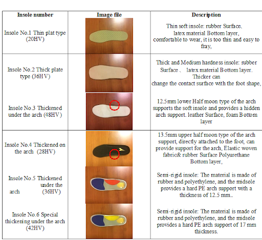
Table 2: Comparison table of Sample insole features.
|
Insole number |
Foot thickness (mm) |
Arch thickness (mm) |
Heel thickness (mm) |
|
InsoleNo1 |
5.2 |
5.2 |
5.2 |
|
InsoleNo2 |
9.5 |
14 |
14.5 |
|
InsoleNo3 |
6.5 |
12.5 |
14.5 |
|
InsoleNo4 |
6 |
13.5 |
11.5 |
|
InsoleNo5 |
5 |
12.5 |
11.5 |
|
InsoleNo6 |
5 |
17 |
11,5 |
Table 3: Sample insole partition thickness.
|
a |
b |
c |
d |
e |
f |
|
Insole No.2 |
Insole No.5 |
Insole No.1 |
Insole No.6 |
InsoleNo.4 |
Insole No.3 |


Table 4: Grey relation sequence of A Testers (six insoles).
|
Insole No.1 |
Insole No.2 |
Insole No.3 |
Insole No.4 |
Insole No.5 |
Insole No.6 |
Fit Insole |
|
|
A tester |
0.815173 |
0.943334 |
0.770541 |
0.803337 |
0.839296 |
0.809525 |
2 |
|
B tester |
0.744014 |
0.974009 |
0.755242 |
0.603723 |
0.763376 |
0.542909 |
2 |
|
C tester |
0.747783 |
0.901872 |
0.701708 |
0.748046 |
0.686388 |
0.756456 |
2 |
|
D tester |
0.671959 |
0.960707 |
0.795055 |
0.727984 |
0.654611 |
0.699062 |
2 |
|
E tester |
0.524422 |
0.899278 |
0.68817 |
0.699428 |
0.739524 |
0.678928 |
2 |
|
F tester |
0.611056 |
0.89952 |
0.689213 |
0.681308 |
0.68019 |
0.831363 |
2 |
|
G tester |
0.669197 |
0.982906 |
0.910551 |
0.757839 |
0.874971 |
0.77478 |
2 |
|
H tester |
0.584233 |
0.961564 |
0.829249 |
0.694132 |
0.613606 |
0.646163 |
2 |
|
I tester |
0.568563 |
0.868096 |
0.807502 |
0.917348 |
0.71679 |
0.714341 |
4 |
|
J tester |
0.60391 |
0.889226 |
0.768586 |
0.639841 |
0.643236 |
0.711983 |
2 |
|
K tester |
0.656198 |
0.87938 |
0.989274 |
0.839595 |
0.731824 |
0.75246 |
3 |
|
L tester |
0.59647 |
0.922816 |
0.78841 |
0.770352 |
0.676498 |
0.783171 |
2 |
|
M tester |
0.767716 |
0.807825 |
0.782753 |
0.704695 |
0.732568 |
0.864776 |
6 |
|
N tester |
0.559733 |
0.863501 |
0.839777 |
0.648558 |
0.737679 |
0.707761 |
2 |
|
O tester |
0.587535 |
0.792212 |
0.790059 |
0.906465 |
0.671046 |
0.717292 |
4 |
|
P tester |
0.671351 |
0.993336 |
0.815081 |
0.758816 |
0.662169 |
0.710241 |
2 |
|
Q tester |
0.679166 |
0.733247 |
0.821136 |
0.86385 |
0.685511 |
0.684502 |
4 |
|
R tester |
0.810604 |
0.943334 |
0.749122 |
0.776918 |
0.794452 |
0.758923 |
2 |
|
S tester |
0.630442 |
0.840333 |
0.94365 |
0.780798 |
0.72011 |
0.722467 |
3 |
|
T tester |
0.575222 |
0.814684 |
0.805749 |
0.721291 |
0.655179 |
0.624268 |
2 |
Table 5: 20 testers calculate Gray relation and optimal insole sorting (six insoles).
|
a |
b |
c |
d |
e |
|
Insole No.5 |
Insole No.1 |
Insole No.6 |
Insole No.3 |
Insole No.4 |


Table 6: Grey relation sequence of A Testers (five insoles).
|
|
Insole No.1 |
Insole No.3 |
Insole No.4 |
Insole No.5 |
Insole No.6 |
Fit Insole |
|
A tester |
0.830811 |
0.814813 |
0.813773 |
0.866137 |
0.817291 |
5 |
|
B tester |
0.859176 |
0.903541 |
0.754529 |
0.833078 |
0.598971 |
3 |
|
C tester |
0.744758 |
0.787211 |
0.791734 |
0.682921 |
0.758246 |
4 |
|
D tester |
0.650377 |
0.920272 |
0.865015 |
0.624398 |
0.723428 |
3 |
|
E tester |
0.505662 |
0.716049 |
0.76913 |
0.746929 |
0.699684 |
4 |
|
F tester |
0.616577 |
0.739706 |
0.793058 |
0.714351 |
0.884497 |
6 |
|
G tester |
0.708257 |
0.965969 |
0.800351 |
0.909625 |
0.81129 |
3 |
|
H tester |
0.602614 |
0.999576 |
0.798845 |
0.637119 |
0.693266 |
3 |
|
I tester |
0.597241 |
0.837411 |
0.939523 |
0.745409 |
0.743188 |
4 |
|
J tester |
0.626713 |
0.910739 |
0.67334 |
0.656151 |
0.724672 |
3 |
|
K tester |
0.654922 |
0.989118 |
0.837623 |
0.729306 |
0.749597 |
3 |
|
L tester |
0.618624 |
0.813089 |
0.795212 |
0.696824 |
0.800855 |
3 |
|
M tester |
0.804377 |
0.820304 |
0.746154 |
0.773245 |
0.905107 |
6 |
|
N tester |
0.579103 |
0.92885 |
0.722335 |
0.763979 |
0.739087 |
3 |
|
O tester |
0.627098 |
0.837256 |
0.951731 |
0.714486 |
0.760365 |
4 |
|
P tester |
0.672912 |
0.96151 |
0.819655 |
0.660346 |
0.729521 |
3 |
|
Q tester |
0.689573 |
0.836576 |
0.89064 |
0.690894 |
0.692523 |
4 |
|
R tester |
0.84744 |
0.803318 |
0.802712 |
0.829916 |
0.773762 |
1 |
|
S tester |
0.644007 |
0.983918 |
0.825085 |
0.740552 |
0.742243 |
3 |
|
T tester |
0.575173 |
0.836336 |
0.795565 |
0.656559 |
0.619998 |
3 |
Table 7: 20 testers calculate Gray relation and optimal insole sorting (five insoles).
|
Epoch |
2000 |
|
Performance Goal |
0 |
|
Learning Rate |
0.01 |
|
neurons |
79 |
|
Momentum Constant |
0.9 |
|
Minimum Performance Gradient |
1.00E-10 |
|
text |
10 |
Table 8: Training parameters.
|
I .tester |
J .tester |
Q. tester |
R tester |
T tester |
||||||||||||||||||
|
Grey Relational Calculated |
4 |
4 |
4 |
4 |
2 |
2 |
2 |
2 |
2 |
4 |
4 |
4 |
4 |
2 |
2 |
2 |
2 |
2 |
2 |
2 |
|
|
|
1 verification |
4 |
4 |
4 |
4 |
3 |
3 |
3 |
4 |
4 |
4 |
4 |
4 |
3 |
4 |
4 |
4 |
4 |
4 |
4 |
4 |
|
|
|
2 verifications |
4 |
4 |
4 |
4 |
3 |
3 |
3 |
4 |
4 |
4 |
4 |
4 |
3 |
4 |
4 |
4 |
4 |
4 |
4 |
4 |
|
|
|
3 verifications |
4 |
4 |
4 |
4 |
3 |
3 |
3 |
4 |
4 |
4 |
4 |
4 |
3 |
2 |
3 |
2 |
4 |
4 |
3 |
3 |
|
|
|
4 verifications |
6 |
3 |
6 |
6 |
3 |
3 |
3 |
4 |
4 |
4 |
4 |
4 |
3 |
3 |
6 |
3 |
4 |
4 |
4 |
4 |
|
|
|
5 verifications |
3 |
3 |
3 |
3 |
3 |
3 |
3 |
3 |
3 |
3 |
3 |
3 |
3 |
2 |
3 |
2 |
3 |
4 |
3 |
3 |
|
|
|
6 verifications |
4 |
4 |
4 |
4 |
3 |
3 |
3 |
4 |
4 |
4 |
4 |
4 |
3 |
2 |
4 |
2 |
4 |
4 |
4 |
4 |
|
|
|
7 verifications |
4 |
4 |
4 |
4 |
3 |
3 |
3 |
3 |
4 |
4 |
4 |
4 |
3 |
4 |
4 |
4 |
4 |
4 |
4 |
4 |
|
|
|
8 verifications |
4 |
4 |
4 |
4 |
3 |
3 |
3 |
3 |
4 |
4 |
4 |
4 |
3 |
2 |
3 |
2 |
4 |
4 |
4 |
4 |
|
|
|
9 verifications |
3 |
3 |
4 |
4 |
3 |
3 |
3 |
3 |
4 |
4 |
4 |
4 |
3 |
3 |
4 |
3 |
4 |
4 |
4 |
4 |
|
|
|
10 verifications |
4 |
4 |
4 |
4 |
3 |
3 |
3 |
3 |
4 |
4 |
4 |
4 |
3 |
3 |
3 |
3 |
4 |
4 |
4 |
4 |
|
|
Table 9: Network a 10 independent program experiments (6 sample insoles).
|
Recognizing accurate |
Gradient |
epoch |
|
|
1 |
40% |
9.56E-11 |
933 |
|
2 |
40% |
9.75E-11 |
674 |
|
3 |
50% |
9.50E-11 |
1135 |
|
4 |
20% |
9.93E-11 |
940 |
|
5 |
10% |
9.93E-11 |
1426 |
|
6 |
50% |
9.87E-11 |
634 |
|
7 |
40% |
9.99E-11 |
1354 |
|
8 |
50% |
9.59E-11 |
856 |
|
9 |
30% |
9.78E-11 |
1175 |
|
10 |
40% |
9.92E-11 |
1173 |
|
average value |
37% |
9.78E-11 |
1030 |
Table 10: Network a. 10 independent program experiments (6 sample insoles).
|
|
I. Tester |
J .tester |
Q. tester |
R. tester |
T .tester |
|||||||||||||||
|
Grey Relational Calculated insole |
4 |
4 |
4 |
4 |
2 |
2 |
2 |
2 |
4 |
4 |
4 |
4 |
2 |
2 |
2 |
2 |
2 |
2 |
2 |
2 |
|
One-time learning verification |
4 |
4 |
4 |
4 |
3 |
3 |
3 |
3 |
4 |
4 |
4 |
4 |
3 |
4 |
4 |
3 |
4 |
4 |
4 |
4 |
|
Recognizing accurate:40.0% |
||||||||||||||||||||
Table 11: Network b learning once - correct rate (6 sample insoles).
|
I .tester |
J. tester |
Q. tester |
R .tester |
T. tester |
||||||||||||||||
|
Grey Relational Calculated insole |
3 |
3 |
3 |
3 |
2 |
2 |
2 |
2 |
3 |
3 |
3 |
3 |
1 |
1 |
1 |
1 |
2 |
2 |
2 |
|
|
1 verification |
3 |
3 |
3 |
3 |
2 |
2 |
2 |
2 |
3 |
3 |
3 |
3 |
1 |
1 |
1 |
1 |
4 |
3 |
4 |
4 |
|
2 verification |
3 |
3 |
3 |
3 |
2 |
2 |
2 |
2 |
3 |
3 |
3 |
3 |
1 |
1 |
1 |
1 |
3 |
3 |
3 |
3 |
|
3 verification |
3 |
3 |
3 |
3 |
2 |
2 |
2 |
4 |
3 |
3 |
3 |
3 |
1 |
1 |
1 |
1 |
3 |
3 |
4 |
3 |
|
4 verification |
3 |
3 |
3 |
3 |
2 |
2 |
2 |
2 |
3 |
3 |
3 |
3 |
1 |
1 |
1 |
1 |
5 |
5 |
5 |
5 |
|
5 verification |
1 |
3 |
3 |
3 |
2 |
2 |
2 |
2 |
3 |
3 |
3 |
3 |
1 |
1 |
1 |
1 |
3 |
3 |
3 |
3 |
|
6 verification |
3 |
3 |
1 |
1 |
2 |
2 |
2 |
2 |
3 |
3 |
3 |
3 |
1 |
1 |
1 |
1 |
1 |
1 |
1 |
1 |
|
7 verification |
1 |
3 |
3 |
3 |
2 |
2 |
2 |
2 |
3 |
3 |
3 |
3 |
1 |
3 |
3 |
3 |
3 |
3 |
4 |
3 |
|
8 verification |
3 |
3 |
3 |
3 |
2 |
2 |
2 |
2 |
3 |
3 |
3 |
3 |
1 |
1 |
1 |
1 |
1 |
1 |
1 |
3 |
|
9 verification |
3 |
3 |
3 |
3 |
2 |
2 |
2 |
2 |
3 |
3 |
3 |
3 |
1 |
1 |
1 |
1 |
2 |
2 |
4 |
2 |
|
10verification |
3 |
3 |
3 |
3 |
2 |
2 |
2 |
2 |
3 |
3 |
3 |
3 |
1 |
1 |
1 |
1 |
2 |
1 |
1 |
1 |
Table 12: Network a successive training results (5sample insoles).
|
Recognizing accurate |
Gradient |
epoch |
|
|
1 |
80% |
9.76E-11 |
818 |
|
2 |
80% |
9.67E-11 |
1437 |
|
3 |
75% |
9.64E-11 |
1024 |
|
4 |
75% |
9.51E-11 |
867 |
|
5 |
80% |
9.55E-11 |
1394 |
|
6 |
65% |
9.55E-11 |
1405 |
|
7 |
60% |
9.93E-11 |
831 |
|
8 |
80% |
1.00E-10 |
1083 |
|
9 |
95% |
9.60E-11 |
711 |
|
10 |
85% |
9.68E-11 |
865 |
|
average value |
77.5% |
9.69E-11 |
1043 |
Table 13: Network a. 10 independent program experiments (5 sample insoles).
|
|
I. Tester |
J .tester |
Q. tester |
R. tester |
T .tester |
|||||||||||||||
|
Grey Relational Calculated insole |
3 |
3 |
3 |
3 |
2 |
2 |
2 |
2 |
3 |
3 |
3 |
3 |
1 |
1 |
1 |
1 |
2 |
2 |
2 |
2 |
|
One-time learning verification |
3 |
3 |
3 |
3 |
2 |
2 |
2 |
2 |
3 |
3 |
3 |
3 |
1 |
1 |
1 |
1 |
1 |
1 |
3 |
1 |
|
Recognizing accurate :80.0% |
||||||||||||||||||||
Table 14: Network b learning once - correct rate (5 sample insoles).
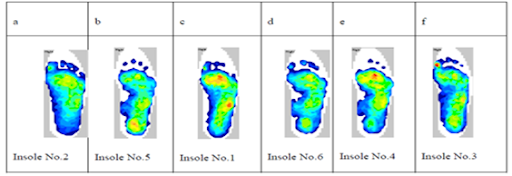
Table 15: Grey Relational ranking of A testers (six insoles).